Porting Postgres histograms to MySQL (MariaDB): Part 2
Welcome to part 2 of the series, in this post, we’ll discuss implementing a new histogram style inspired by Postgres in MySQL for estimating row selectivity.
By now I am assuming you have understood what is selectivity and its significance. If not, I’d recommend you to read part 1 for this post to make sense.
TLDR 🏃
In the last post, you noticed how postgres utilizes bounds to create its histogram implementation. I decided to utilize the same idea with a small twist to implement a new histogram style in MySQL called RANGE_HB (to be fair, I could’ve thought of a better name but I was half asleep and caffeinated through most of this hack week xD). You can check out the implementation in this branch:
It seems to be giving a better selectivity ratio than both existing MySQL and Postgres implementation (on a sample of 1 table only btw, so don’t take my word for it 😅)
A new histogram
Without further ado, let’s build a new histogram.
For my implementation, I want to merge both ideas, that is, I’ll maintain histogram bounds as the endpoints of a bucket, and in the buckets, I’ll put average running sum (running sum / total sum) instead of assuming equidistant values. To achieve this, I’ll need two things at the point of histogram creation.
- I’ll need the minimum and maximum column values and the histogram width, so typically, the bound would range in
(max-min)/histogram widthsize. - I’ll need the frequency of appearance of all the different values.
Once these conditions are satisfied, my histogram should be able to do three basic things:
- Estimate the range_selectivity between two different values.
- Estimate the point_selectivity for a particular value (query planner uses that for estimating constant queries)
- I should be able to print this histogram!
Lifecycle of a histogram for a column
Before we jump into our data structure, let’s try and understand the auxiliary existing ones.
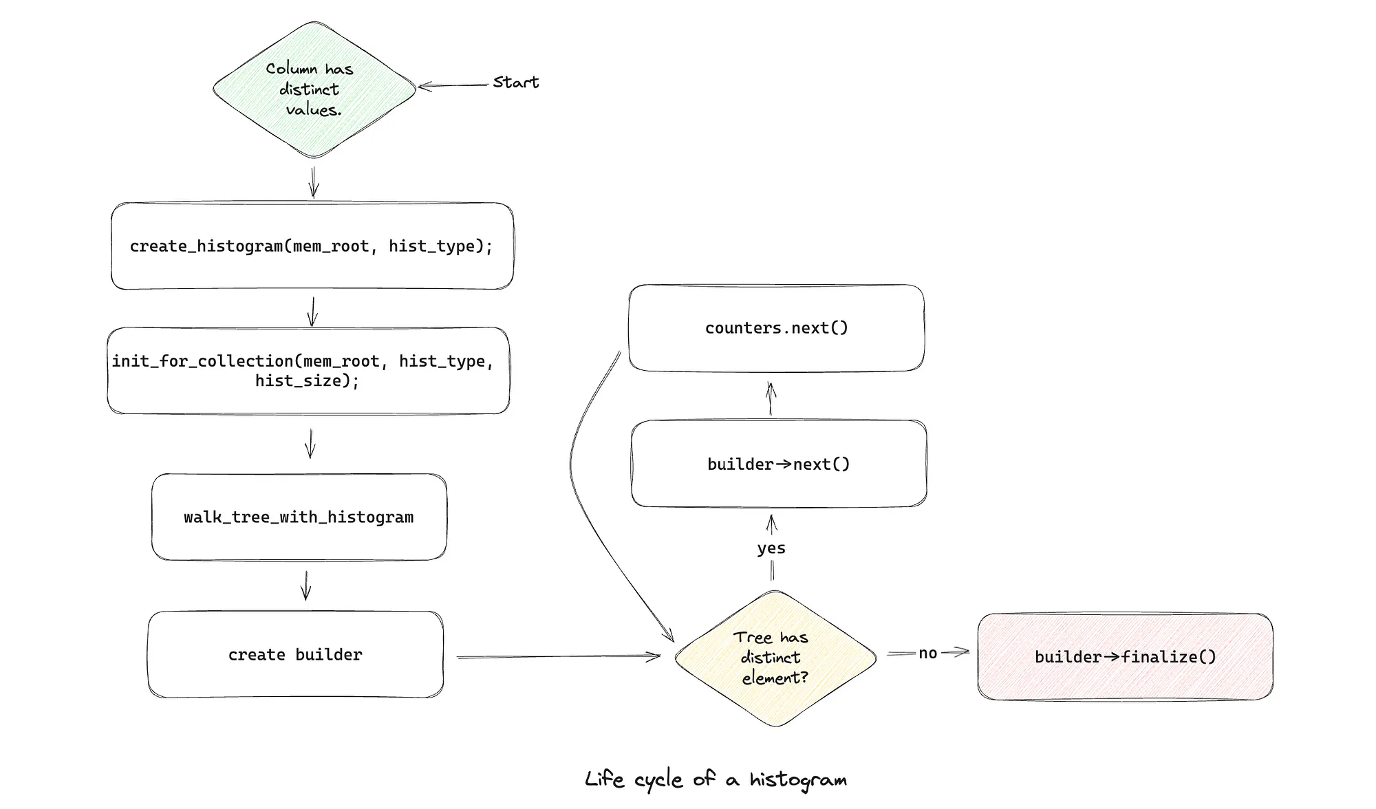
MySQL columns create a tree that maintains the element and the frequency of these elements. For histogram creation, we need to follow a certain lifecycle (described in the image), during the walk_tree_with_histogram step, we maintain the relevant frequency data in a counter of sorts before finalizing the histogram!
This walk_tree_with_histogram runs on top of an internal data structure that uniquely holds elements and their frequency in a tree form.
Building the histogram
With the lifecycle out of the way, let’s focus on how would we create one. Histogram_baseis the base class that any histogram has to implement, and our binary will be implementing the same.
class Histogram_range_binary final: public Histogram_base {

  Histogram_type type;
  size_t size; /* Size of values array, in bytes */
  uchar *values;

  public:
    Histogram_range_binary() {
      type = RANGE_HB;
    }

    uint get_width() override
    {
      return size;
    }

    uint get_size() override
    {
      return (uint)size;
    }

    Histogram_type get_type() override {return type;}

    bool parse(MEM_ROOT *mem_root, const char*, const char*, Field*,
             const char *hist_data, size_t hist_data_len) override ;
    void serialize(Field *to_field) override;
    void init_for_collection(MEM_ROOT *mem_root, Histogram_type htype_arg,
                            ulonglong size) override ;
    Histogram_builder *create_builder(Field *col, uint col_len,
                                      ha_rows rows) override;

    double point_selectivity(Field *field, key_range *endpoint,
                           double avg_sel) override;
    double range_selectivity(Field *field, key_range *min_endp,
                           key_range *max_endp, double avg_sel) override;

    void set_value(uint i, double val) {
      ((uint8 *) values)[i]= (uint8) (val * ((uint) (1 << 8) - 1));
    }

  private:
    double get_value_double(uint i)
    {
      DBUG_ASSERT(i < get_width());
      return (((uint8 *) values)[i]) / (double) ((1 << 8) - 1);
    }
};
To give a brief introduction to this class, Histogram_range_binary will be utilizing an array of uchar values. Every time a double value has to be set on a certain index, I’ll be setting it as a uint8 , essentially multiplying the value to (1<<8)-1 (see set_value and get_value_double).
I could’ve used the double* array directly but later on when calculating the range selectivity, it seems that the memory address where I was storing the data, over there some garbage value was re-written, so I decided to hack around and borrow the implementation done by SINGLE_PREC_HB.
Now, once the binary is sorted, we still need to create a builder no? For my use case, I built Histogram_range_builder
class Histogram_range_builder : public Histogram_builder {
  Advanced_stats_collector advanced_counter; // Init the new advanced counter here.
  Field *min_value;        /* pointer to the minimal value for the field   */
  Field *max_value;        /* pointer to the maximal value for the field   */
  Histogram_range_binary *histogram;  /* the histogram location                  */
  uint hist_width;         /* the number of points in the histogram        */
  uint curr_bucket;        /* number of the current bucket to be built     */
  uint curr_ptr;           /* current pointer to tack position */
public:
  Histogram_range_builder(Field *col, uint col_len, ha_rows rows)
    : Histogram_builder(col, col_len, rows)
  {
    Column_statistics *col_stats= col->collected_stats;
    min_value= col_stats->min_value;
    max_value= col_stats->max_value;
    histogram= (Histogram_range_binary*)col_stats->histogram;
    hist_width= histogram->get_width();
    curr_bucket= 0;
    curr_ptr = 0;
  }

  int next(void *elem, element_count elem_cnt) override
  {
    counters.next(elem, elem_cnt);
    advanced_counter.next(elem, elem_cnt);
    column->store_field_value((uchar *) elem, col_length);
    double position_in_interval = column->pos_in_interval(min_value, max_value);
    advanced_counter.push_pos(position_in_interval);
    return 0;
  }
}
Here, as you can notice, it also extends a Histogram_builder base class which contains a basic counter. Largely, you need to understand that this class has a Advanced_counter which stores the relative position of the element in the tree ( (element-min) / (max-min) ) and its frequency in two separate arrays, while the basic stat counter, counters will be storing the total running count, the number of distinct elements, and the number of elements with only single values.
Once we have gathered all the data, we will be building the actual histogram in the final step of a histogram lifecycle, called finalize() . The code might look a bit complicated (fairly because it's not clean code perse) but on a high level, it’s a two-pointer algorithm.
We’ll go through all the values collected, and see if the current element’s position is within the bucket, if it’s within the bucket then we increase the running sum. If it’s not within the bucket, then we set the running sum to the appropriate bucket, and move the bucket forward till it matches our pointer!
void finalize() override
{
  // here build the histogram.
  double bucket_range = 1.0 / hist_width;

  ulonglong distinctValues = counters.get_count_distinct();
  ulonglong totalCnt = counters.get_count();

  double default_val = 0.0;
  double pos_min = bucket_range * curr_bucket;
  double pos_max = bucket_range * (curr_bucket+1);
  double running_pos;
  if (pos_max > 1.0) {
    pos_max = 1.0;
  }

  ulonglong runningSum = 0;
  for (curr_ptr=0; curr_ptr<distinctValues; curr_ptr++) {
    double curr_pos = advanced_counter.pos_at(curr_ptr);
    if (curr_pos >= pos_min && curr_pos < pos_max) {
      runningSum += advanced_counter.frequency_at(curr_ptr);
      running_pos = curr_pos;
    } else if (curr_pos == pos_max && curr_ptr == distinctValues-1) {
      // last bucket.
      if (curr_pos != running_pos) {
        while (curr_bucket != hist_width && pos_max < curr_pos && pos_max != 1.0) {
          if (running_pos >= pos_min && running_pos < pos_max) {
            double val = (double)runningSum / totalCnt;
            histogram->set_value(curr_bucket, val);
            runningSum = 0;
          } else {
            histogram->set_value(curr_bucket, default_val);
          }
          curr_bucket++;
          pos_min = bucket_range * curr_bucket;
          pos_max = bucket_range * (curr_bucket+1);
          if (pos_max > 1.0) {
            pos_max = 1.0;
          }
        }
      }
      runningSum += advanced_counter.frequency_at(curr_ptr);
      running_pos = curr_pos;
    } else {
      // we need to fill the buckets with runningSum till pos_max is again > curr_pos
      while (curr_bucket != hist_width && pos_max < curr_pos && pos_max != 1.0) {
        if (running_pos >= pos_min && running_pos < pos_max) {
          double val = (double)runningSum / totalCnt;

          histogram->set_value(curr_bucket, val);
          runningSum = 0;
        } else {
            histogram->set_value(curr_bucket, default_val);
        }
        curr_bucket++;
        pos_min = bucket_range * curr_bucket;
        pos_max = bucket_range * (curr_bucket+1);
        if (pos_max > 1.0) {
          pos_max = 1.0;
        }
      }
      if (curr_pos >= pos_min && curr_pos <= pos_max ) {
        runningSum += advanced_counter.frequency_at(curr_ptr);
        running_pos = curr_pos;
      }
    }
  }
  if (curr_ptr == distinctValues) {
    double val = (double)runningSum / totalCnt;
    histogram->set_value(curr_bucket, val);
    curr_bucket++;
  }
}
Implementing the range_selectivity()
Once the histogram is built, we have to implement the actual range selectivity. I have borrowed the existing histogram algorithm to find the relative position of the elements.
After that, I try and figure out the buckets that will be the bounds for the minimum and maximum position (again, could’ve used a binary search but since the maximum histogram width itself is 256, why bother optimizing an O(1)? ) Once they are found, all we need to do is add up the values present in each bucket and return that.
double Histogram_range_binary::range_selectivity(Field *field, key_range *min_endp, key_range *max_endp, double avg_sel) {
  double sel, min_mp_pos, max_mp_pos;
  Column_statistics *col_stats= field->read_stats;

  if (min_endp && !(field->null_ptr && min_endp->key[0]))
  {
    store_key_image_to_rec(field, (uchar *) min_endp->key,
                           field->key_length());
    min_mp_pos=
        field->pos_in_interval(col_stats->min_value, col_stats->max_value);
  }
  else
    min_mp_pos= 0.0;
  if (max_endp)
  {
    store_key_image_to_rec(field, (uchar *) max_endp->key,
                           field->key_length());
    max_mp_pos=
        field->pos_in_interval(col_stats->min_value, col_stats->max_value);
  }
  else
    max_mp_pos= 1.0;

  double bucket_range = 1.0 / get_width();
  uint bucket, bucket_min, bucket_max;
  for (bucket=0; bucket < get_width(); bucket++) {
    double min_pos = bucket_range * bucket;
    double max_pos = bucket_range * (bucket + 1);
    if (max_pos > 1.0) {
      max_pos = 1.0;
    }
    if (min_mp_pos >= min_pos && min_mp_pos < max_pos) {
      bucket_min = bucket;
    }
    if (max_mp_pos >= min_pos && max_mp_pos < max_pos) {
      bucket_max = bucket;
    }
  }

  if (max_mp_pos == 1.0) {
    bucket_max = get_width() - 1;
  }
  if (min_mp_pos == 1.0) {
    bucket_min = get_width() - 1;
  }

  sel = 0.0;
  for (uint i = bucket_min; i<=bucket_max; i++) {
    sel += get_value_double(i);
  }
  sql_print_information("[histogram_range_binary::range_sel] avg_sel: %f, range_sel: %f", avg_sel, sel);
  set_if_bigger(sel, avg_sel);
  return sel;
}
Estimation Accuracy
The algorithm sounds good but let’s see how it performs. I’ll be building a similar table which we used in the last example to check the selectivity given by this histogram.
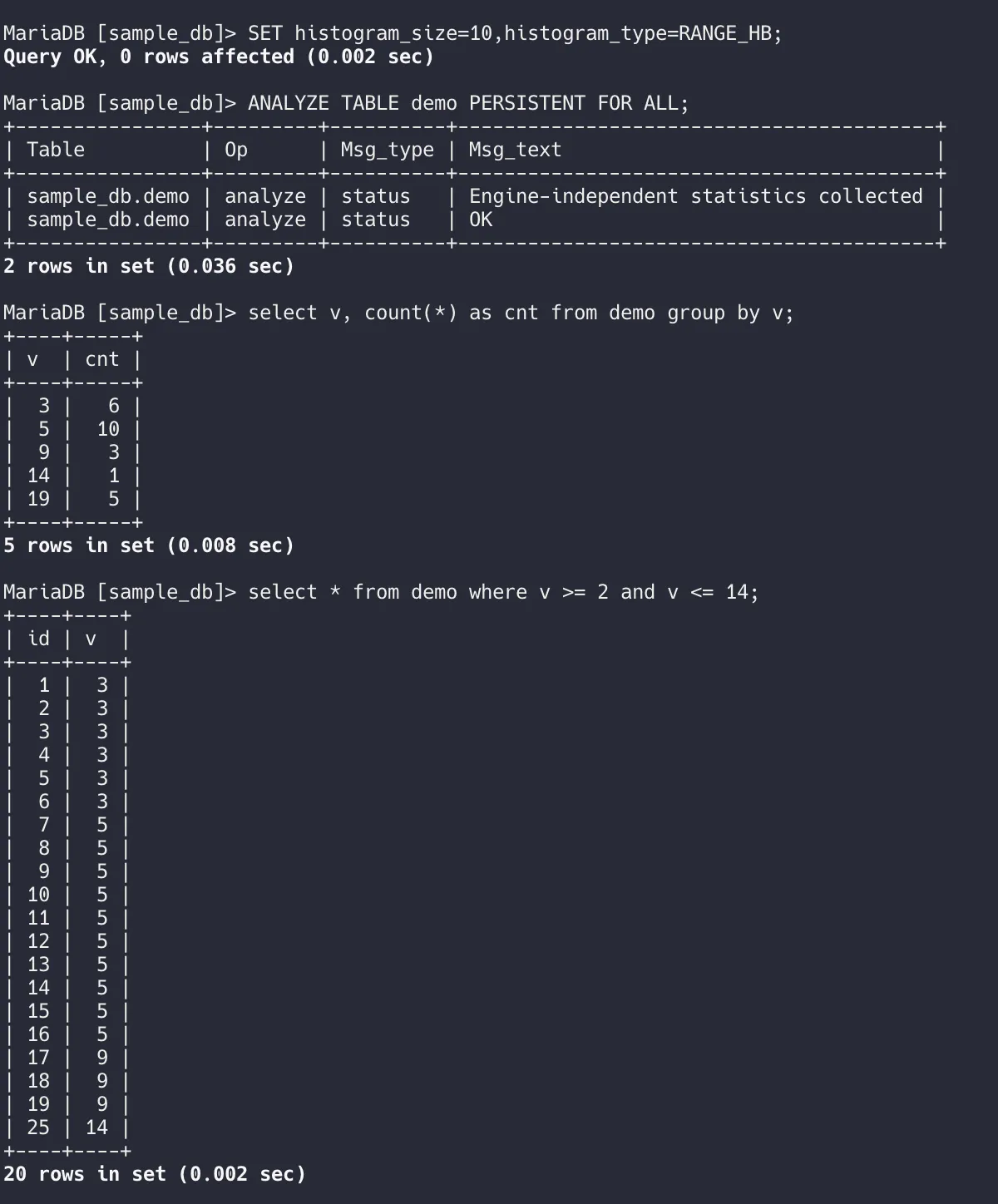
The demo table above is using RANGE_HB histogram with size 10.
However, the selectivity is ~0.8 in our histogram’s case, which means it’ll suggest the query planner to return 0.8 * 25 = 20 rows instead of 18 in the other two implementations, which means that this implementation gives more accurate estimations! (For this use case at least)

Displaying the histogram
The math is done, now time to show the world what we are doing. I modified the existing display function to show actual values on each bucket instead of the delta of the last bucket (you can check out the implementation in the GitHub repository linked at the top).
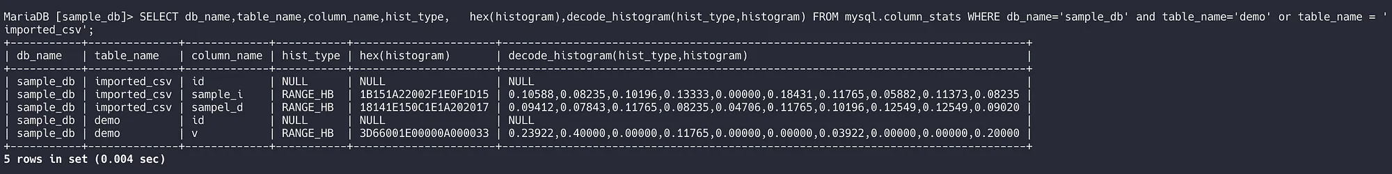
For the sake of this demo, I created another table imported_csv and used the histogram there as well, as you can see in the buckets where there is no value, the sum is plain 0.000 !
Caveats (Disclaimers)
While the implementation looks smooth, like Andy Pavlo says, there are no free lunches in software engineering!
There are a couple of bugs where I am not sure how this histogram or the server itself will behave, let’s talk about them.
- In the native implementations, you didn’t need each position and frequency separately, you just needed a running sum of the elements which ensured that your builder didn’t consume an array worth of memory. In my implementation, with the introduction of 2 vectors in the
Advanced_Counter, it might consumer instance/program memory when there are let’s say millions of distinct values. - During the
walk_tree_with_histogramstep, it’s required to delete the histogram builder pointer and free up that memory manually. Due to some issue, this memory pointer was already deallocated before I could free it up myself. For now, the pointer deletion has been commented out… so, after a few large histograms, your server is bound to crash in the current state. (welp! send a fix if anyone can help 😢)
Conclusion
In all, this hack helped me gain a deeper insight and appreciation of how query planner internally functions in MySQL source and how could I help it estimate the row selectivity slightly better with tradeoffs! I’ll mess around with its kernel while trying to solve an existing issue in the future maybe, for now, adios!