Porting Postgres histograms to MySQL (MariaDB): Part 1

A more accurate title would’ve been porting Postgres’ conditional selectivity to MySQL, but you’d ask me what’s conditional selectivity then! This blog post series will explain both.

Introduction

I have been hacking around since last week in MySQL/MariaDB hack week (organization courtesy — Phil!) with ~80 odd brilliant hackers. Going into the hack week, my goal was to figure out how a SELECT query works in MariaDB and how its Query Execution Planner(QEP) internally works.

The rough notes that I took through the week around QEP notes can be found here in this gist.

Edit : If you already know about selectivity concept in databases thoroughly, you can skip to part 2, to the actual implementation.

During my QEP code read, I realized that all the plans are built around pre-calculated statistics for Tables, Indexes, and Columns (in MySQL). These plans may sometimes utilize histograms to determine the selectivity of rows on un-indexed columns, while I can’t change the QEP algorithm in a week, I sure as hell can implement some data structures! But before we get there in the implementation details, let’s address the elephant in the room.

What’s Selectivity?

Imagine you have the following table

CREATE TABLE sample_table (
  id INT PRIMARY KEY AUTO_INCREMENT,
  i INT NOT NULL,
  d DOUBLE NOT NULL);

CREATE_TABLE sample_inner_table {
  id INT PRIMARY KEY AUTO_INCREMENT,
  i INT NOT NULL,
}

CREATE INDEX sample_table_d on sample_table(d);

// Imagine sample_table &sample_inner_table has 20,000,000 rows.

Now, imagine you run the following query

SELECT sample_table.id,sample_inner_table.id AS inner_id
FROM sample_table
JOIN sample_inner_table ON sample_table.i = sample_inner_table.i
WHERE sample_table.d > 10.0
  AND sample_inner_table.id > 5
  AND sample_table.i = 3;

Your database’s query planner will try and estimate the following query plans (among other plans)

Sample plan by QEP

To estimate the IO Cost and the number of rows it’ll need to pass on to the join in Select predicates, i.e, σ(id>5) and σ(i=3 AND d>10), your database can either use indexes (which it’ll most probably use for σ(d>10)) or it will use existing histograms / similar data structures to determine how many rows I want to send to the next step, this ratio is called selectivity.

Rows sent to the next stage would be selectivity * total_rows

You can learn more about it in CMU’s F2023 #14 — Query Planning & Optimization

F2023 #14 — Query Planning & Optimization

How does MariaDB/MySQL do it?

As of MariaDB 11.4, there are 3 histogram implementations, two of them are height-balanced (SINGLE_PREC_HB and DOUBLE_PREC_HB) and by default, they use somewhat new JSON_HB (I have a hunch this is already similar to postgres, based on the values but I haven’t checked it’s implementation :) )

Fun Fact: JSON_HB was introduced as a Google Summer of Code Project, as per this JIRA.

I will currently take the example of SINGLE_PREC_HB and explain how histogram building works in its context.

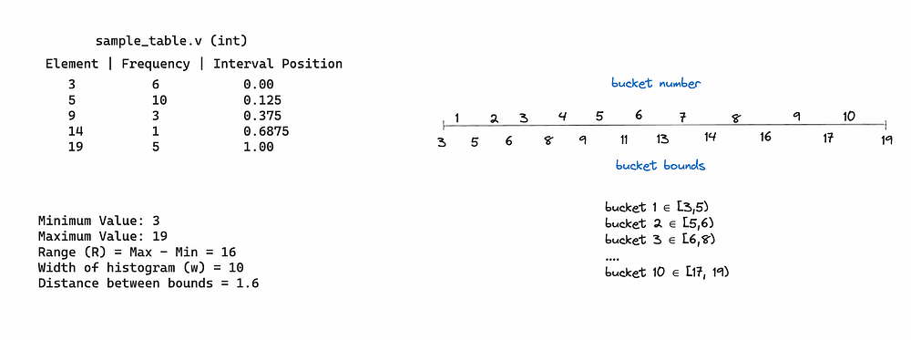
Imagine the total rows in the table to be R, and the histogram width to be w, so each bucket in the histogram would take R/w records. In the bucket, however, you’ll be storing the relative position of the current element where the relative position is determined by (current_element-min_element)/(max_element-min_element) in the column.

The image below should make more sense 😄

Histogram built by MySQL in SINCLE_PREC_HB

You can find the algorithm of histogram building below but as an overview, if the current cumulative row count > bucket * capacity, then I’ll set the interval position in this bucket otherwise I’ll proceed to the next distinct element.

Ex: The cumulative count while processing Element 9 would be 6 + 10 + 3 (16).

Histogram_binary_builder::next()· MariaDB/server

Now, when you are running the query:

SELECT * FROM sample_table WHERE v >= 2 and v <= 14; 

It’ll convert 2 and 14 to respective estimated positions (here, they’ll be 0.00 and 0.6875 respectively). Now, you’ll try and find the buckets where these values can lie. So, your min bucket index will be 1, and the max bucket index will be 7. Hence the planner can send you rows stored in an estimated 7 buckets!

Since you have a total 10 buckets, the selectivity becomes 7/10 or 0.700 and the QEP will be returning an estimated 0.700*25 = 18 rows.

This way of estimating selectivity is called range_selectivity!

Sweet! But how does postgres do it?

Postgres handles different kinds of data types differently, but to keep this discussion simple, we’ll stick with integers. To read the implementation detail better, I’d suggest reading this row estimation algorithm.

Unlike MySQL, postgres distributes its buckets to hold different value bounds.

postgres histogram bounds

If you notice here, we don’t talk about the frequencies of the element appearing 🤔. We just assume that all the buckets have equal chance of appearing (as MySQL does) and selectivity of an element in a bucket is determined by (element — min_bound) / (max_bound-min_bound) , sounds familiar no? 😉

That being said, let’s estimate what happens when we run the query:

SELECT * FROM sample_table WHERE v >= 2 and v<=14;

As we can see, v≥2 and v<= 14means buckets 1–7 will be completely included in this range and bucket 8 will be partially included.

So, the selectivity shall be (7+(0/2))/10 = 0.700

Funny how the selectivity turns out to be the exact same in both histogram layouts no? 🚀

Conclusion

I hope you now understand selectivity! I’ll request you to go and play around with this concept first before we move on to the porting implementation details in the next blog post.