Mathematical Intuition of Phi φ Accrual Failure Detection
In 2004, Naohiro Hayashibara [Et. al] released Phi Accrual Failure Detection paper. This post will elaborate on the goals of this detector, the design, and underlying mathematical principles to understand this beautiful yet simple algorithm!
Introduction
Before the maths, let’s understand why we even need accrual detectors.
Imagine you have a distributed system with a master process monitoring a bunch of worker processors (imagine master <> slave replica setups in your common databases). For the master node to know that the slave is still up and running and can be allocated tasks, it needs to know if the slave is even up and running or not.
If you have been playing with any distributed system, it’s natural to imagine that heartbeats fit the bill for this use case. In Sections II C and D the authors touch base on heartbeat & adaptive detectors (which utilize heartbeats internally!).
The underlying issue for both of these detectors is their incapability to handle scenarios where let’s say your heartbeat timeout is configured to be 1000ms and the worker fails to give any response before 1005ms. The detectors would assume the slave to be down which is actually up and running.
These detectors answer in a binary (0/1) fashion, leaving no room for ambiguity. Either system is up or it is not, there’s nothing in between. This is where your accrual detectors shine by providing the probability of the system being down.
By the way, if you’re here to play around with this detector, I would recommend you to check out my rust implementation for the same with the provided source code 😃
Uncovering the magic of probability
The probability of whether the system is down or not can be termed suspicion (φ) which is dependent on the probability of whether the master would receive any heartbeat after the current time.
In the paper, the authors have stored the last 1000 (sample window space) intervals, the mean & variance of this sample space, and the timestamp of the last heartbeat/ping received by the master. Additionally, they assume that this sample space comprising of inter-arrival time differences follows a normal distribution. With these in mind, they have mentioned the following definitions:

There’s too much for stats novices (like me) to take in at once. So let’s pause. Let’s try and slowly build up our intuition how do we even get to the formula at (3) and what do these terms mean? The following subpoints will explain the relevant concepts sequentially leading up to the derivation of the above formula.
Note: Medium does not have the best maths support hence I’ll be attaching screenshots and links to corresponding matcha documents.
[A] Continuous Random Variable
A random variable is a variable whose value is unknown or a function that assigns a value to each experiment’s outcome. It could have a discrete value at a particular point (discrete random variable) or it could have a continuous value across a range.
You could imagine the snowfall record of a city throughout the year as a continuous variable because, on some days the snowfall might’ve been 5ft, 3.4 ft, 0 ft, etc hence taking continuously infinite values. However, a more accurate definition of a continuous random variable would be that if any random variable could be described by a probability density function (PDF), then it’s continuous.
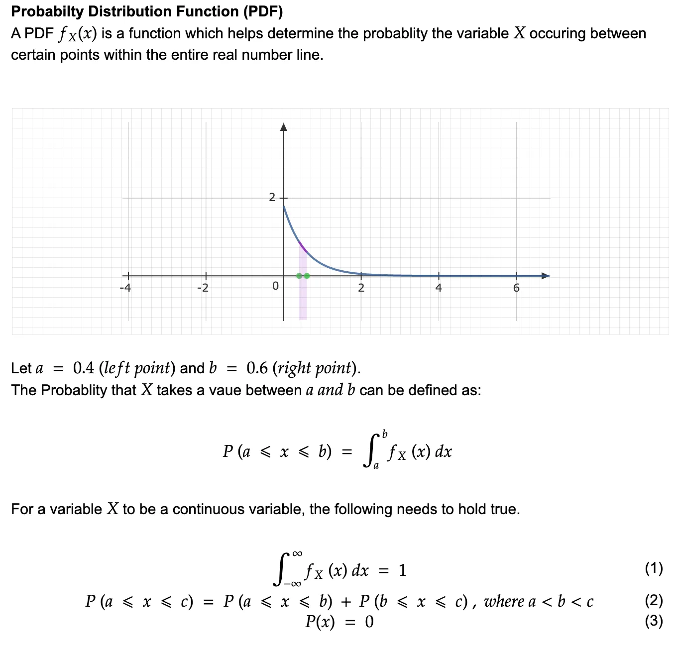
A PDF can be imagined as a function of probability for some variable X that is spread throughout the real line but the sum of all the probabilities across all the values X could take is 1. Kindly refer to the notes mentioned below to understand PDFs and continuous random variable definitions. (In the example, we have taken an exponential continuous distribution)
[B] Cumulative Distributive Function (CDF)
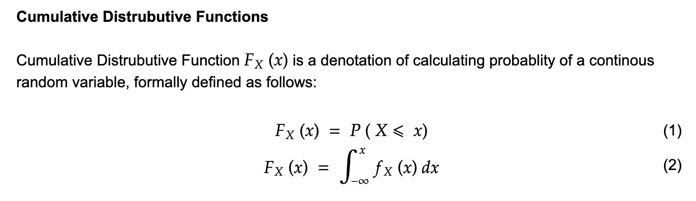
This would be the easiest one to explain by far, a CDF is an expression that denotes the probability of a random variable (both continuous and discrete) to appear than a particular value(let’s say x) on the real line. More formal denotation is described in the image below:
[C] Normal Distribution (Gaussian distributions)
Another new term! hold on, we are so close to glory 😅.
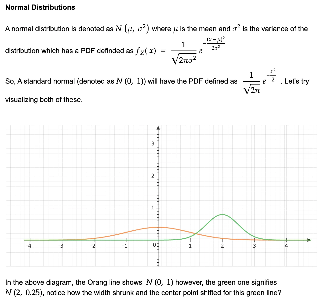
You must’ve seen this bell curve distribution when it comes to denoting metrics that have the majority of values centered around their mean and the probability of that value reduces as you move out further away from the mean.
The derivation of standard normal is tricky and I believe this math overflow question helps the best to get the intuition of its derivation. For our research paper’s derivation purpose, we’ll take it as a given that a normal distribution’s PDF will be denoted by N(mean, variance).
Derivation
With the three concepts above, we are now equipped to derive our suspicion (φ)!
We will start by visualizing the sample space, let’s say for all the last 10000 incoming heartbeat intervals, you get the mean as 3 and variance as 0.04. Assuming a normal distribution, the graph would look somewhat like this:
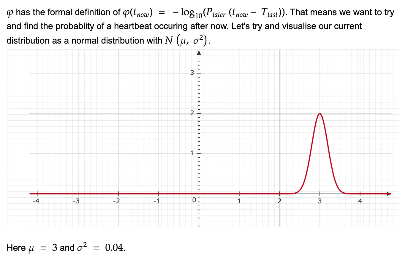
Now, assume that your last heartbeat was received at some time 96.8s and you want to check the suspicion of the system being down at 100s (basically, 3.2s after the last ping). That just means we want to get the probability under the shaded region as shown in the picture below.
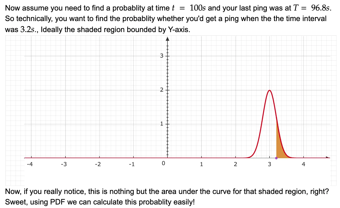
Using this intuition, we’ll now redefine phi step by step as mentioned below

(1) is the basic definition of suspicion while (2) is derived from the definitions of PDF that the sum of all probabilities across the real line for the variable should be 1. Additionally, we can break the entire real line from (-inf, inf) to (-int, t) + (t, inf) as shown in (3).
Great, now remember we defined P(x ≤ t) as a Cumulative distributive function? Let’s leverage that in (4). Steps (5) and (6) are basic algebra. In step (7), we’ll just expand the CDF using the PDF of this normal distribution and plug it in (8). Tada! your implementation can choose whatever flavor it wants out of the two mentioned in the end 😄
Conclusion
By this blog, I hope you achieved a better grasp of random variables and how to decipher basic mathematical derivations in the failure detector research papers (and hopefully others).
If you wish to go deeper into detail regarding how to choose the suspicion value to take action on, what’s an ideal detector, and so on, I’d recommend skimming through the paper, it’s an amazing read in itself.